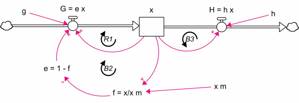
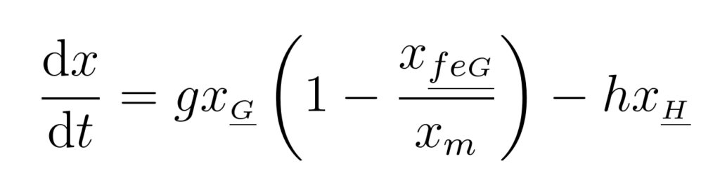
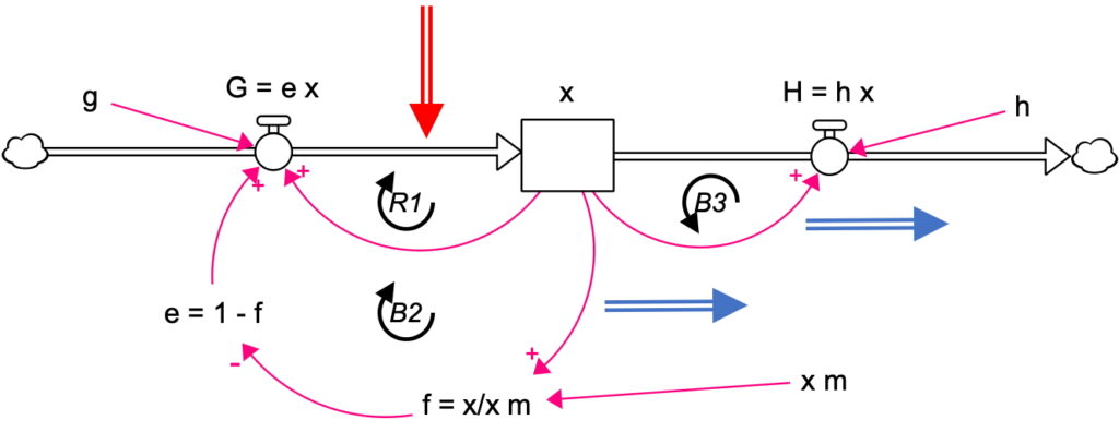
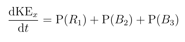
The three-loop Limits to Growth model can be presented in stock-flow form and as a differential equation in causal form:

Using the loop impacts (see loop impacts), the differential equation can be converted into a power balance equation that describes how the loops inject and remove energy from the stock. Loops are measured by their power (energy per unit time), with the changes in the stock represented by its kinetic energy.

Kinetic Energy

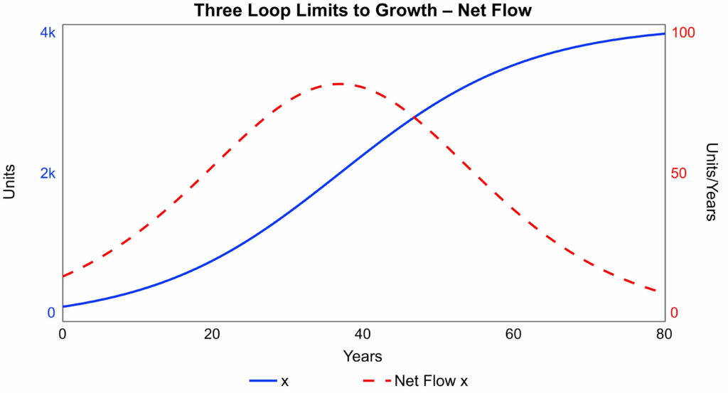
The net flow of stock $\dot{x}$ measures how quickly the stock changes over time. It measures stock activity. The higher the net flow, the more the stock changes, that is, the more the stock is active. If the netflow is zero, then the stock is not changing at that time, that is, it is inactive. Figure 2 compares the net flow with the stock value in the Limits to Growth model. The net flow peaks at the inflexion point of the stock. It tends to zero as the stock reaches equilibrium.

A more useful measure of stock change or activity is its kinetic energy as this will satisfy a conservation law with the loops. Kinetic energy is defined as:

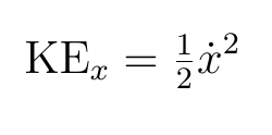
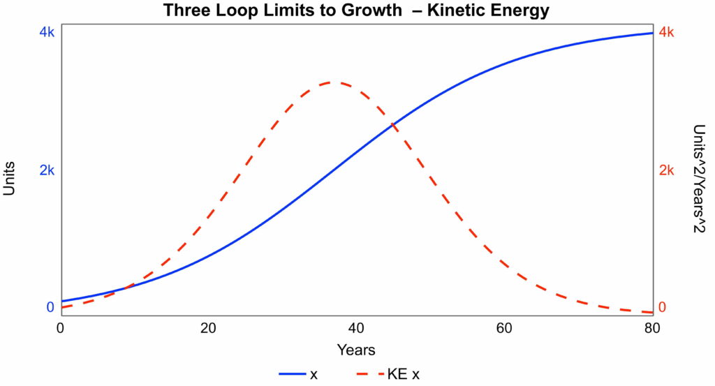
Figure 3 compares the stock with its kinetic energy. The kinetic energy gives a description of the net flow. The advantage of kinetic energy is that it satisfies a conservation law and can be decomposed into energy flows to and from its three feedback loops.

Energy Flows

To obtain the energy flows in this mode, use the impact equation connected with the model (derived in Loop Impacts equation 6), then multiply by $\dot{x}$:

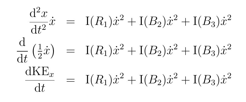
The third equation in equation 3 is the power balance equation showing how the stock’s kinetic energy is changed by the three feedback loops. The three terms on the RHS are the powers of the three loops:

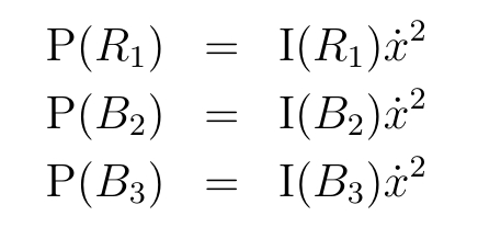
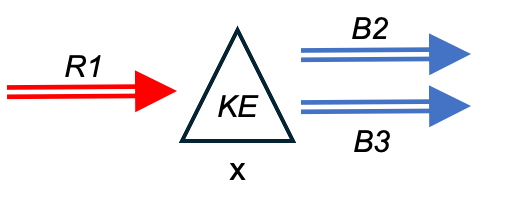
The loop powers are proportional to the impacts. As I(R1) is positive, the reinforcing loop injects energy into the stock. The two balancing loops have negative impacts and remove energy from the stock. These energy flows can be placed on the stock flow diagram of Figure 1, see Figure 4:

At any given time, the three energy flows may not be in balance. The excess energy flows are either injected or removed from the stock’s kinetic energy, shown in Figure 3.

Power Analysis

Using the loop impacts (Loop Impacts equation 3), the loop powers are plotted over time, Figure 5. The regions of loop dominance for power are identical to those for loop impact due to their proportional relationship, equation 3. Initially, the energy injected by R1 dominates, and the kinetic energy of the stock rises (Figure 3). That is, the stock accelerates. The power of R1 starts declining before the balancing loops become more powerful. Thus, the transition occurs because the balancing loops become more powerful, and the reinforcing loop becomes less powerful

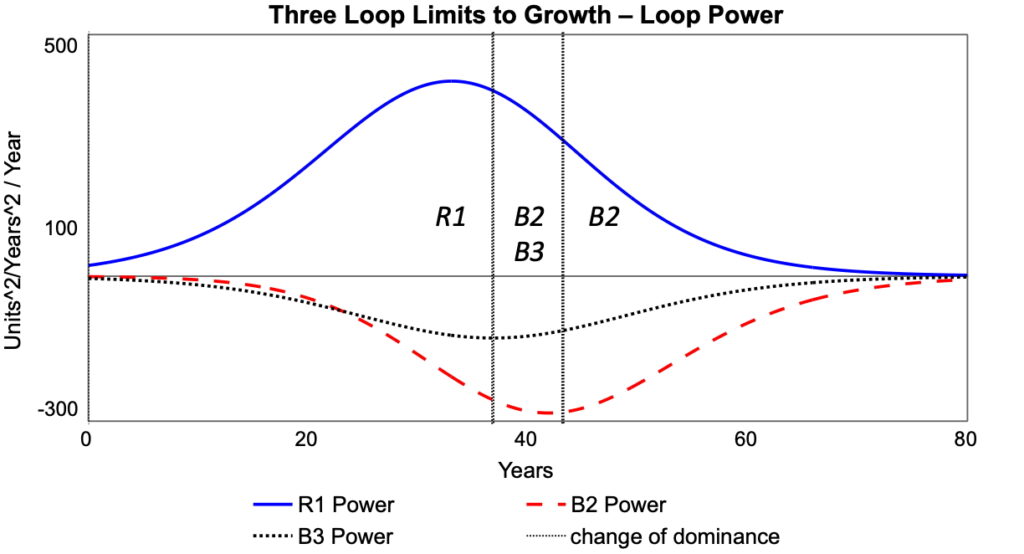
Early in the run, the depletion loop B3 is slightly more powerful than B2. However, B2 eventually becomes more powerful for these parameter values. With a high depletion rate $h$, B3 will become the most powerful loop.

Power Balance Equation

The power balance equation (third of equation 3) may be rewritten using the loop powers (equation 4):

Equation 5 is an alternative to the equation of motion, the differential equation, (equation 1), providing an energy-flow viewpoint of the Limits to Growth model. This equation can be represented as a diagram, Figure 6, linking the energy flows of the loops to the kinetic energy of the stock $x$, represented by the triangle. The power balance is at the heart of the Newtonian Interpretive Framework, which views system dynamics models in Newtonian terms.

References

1. Hayward J, Roach PA. 2017. Newton’s Laws as an Interpretive Framework in System Dynamics. System Dynamics Review, 33(3-4), 183-218.  DOI: 10.1002/sdr.1586.
2. Hayward J, Roach PA. 2019. The Concept of Force in Population Dynamics, Physica A: Statistical Mechanics and its Applications, 531, 121736, DOI: 10.1016/j.physa.2019.121736.
3. Hayward J, Roach PA. 2022. The Concept of Energy in the Analysis of System Dynamics Models, System Dynamics Review, 38(1), 5-40. DOI: 10.1002/sdr.1700