This example illustrates the effects of loop impact in a limits-to-growth model.
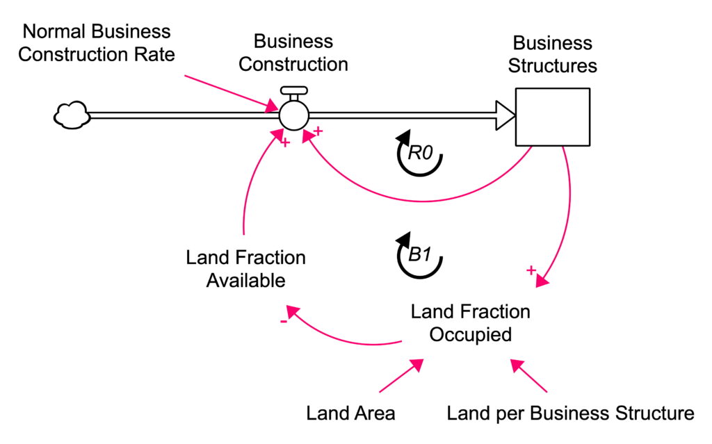
A fixed amount of land is designated for a new trading estate to encourage business development in a town. Initially, the trading estate grows rapidly as more businesses attract further business developments, the urban attractiveness hypothesis R0. However, as growth continues, land availability falls, and business construction is reduced, B1. The model is first-order. See Figure 1.
Simulating the model shows the classic S-shaped growth (Figure 2). Comparing the loop impacts of the two loops shows that the reinforcing loop R0 dominates as the growth in Business Structures accelerates. Once that growth slows down, loop B1 dominates. This is classic “shifting loop dominance”. Dominance shifts from the reinforcing loop (accelerating) to the balancing loop (decelerating).

Loop Impact
The values of the loop impacts are compared in Figure 3. The units are “per year”. The impact of R0 on Business Structures is positive and decreases over time. First-order reinforcing loops have a positive impact, as loop impact has the same sign as loop gain in first-order loops. By contrast, the impact of B1 on the stock is negative and increases in absolute value. Thus, R0 gets weaker while B1 gets stronger. Therefore, B1 eventually has a greater impact than R0 (in absolute terms). The loop with the greater impact has the most influence on the curvature in the stock graph. The model is non-linear due to multiplication in the flow Business Construction. Thus, both loops are non-linear, which is why their impacts change over time.

Three-Loop Limits-to-Growth
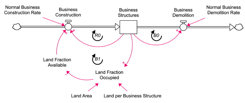
If buildings are demolished at a fixed rate, then a third loop, B0, is added, as shown in Figure 4. This loop is balancing and linear, depleting the stock—a draining process.
There are now three loops influencing stock behaviour. Initially, R0 dominates, the accelerating phase, until the combination of B1 and B0 has a larger impact, as shown in Figure 5. In this middle phase, no single loop dominates. R0 still has the largest impact of the three loops, but the sum of the two balancing loops is larger than that of R0 – hence, the stock growth is slowing down. In the third phase, B1 has the largest impact, thus dominates over R0.

The impacts of the three loops are compared in Figure 6. As loop B0 is linear, its impact is constant (green dotted line). Initially, loop B0 has a larger impact than B1, but this phase has no noticeable effect on stock behaviour as both loops are decelerating. In the middle phase, where it takes both B0 and B1 to dominate over R0, the value of B0‘s impact has enabled B1 to slow the growth earlier than would have happened if there had been no demolition. Thus, demolition shortens the acceleration phase. Demolition also lowers the carrying capacity, seen in the maximum value of Business Structures, compare figures 2 and 5.
