The three-loop Limits to Growth model can be presented in stock-flow form and as a differential equation in causal form:
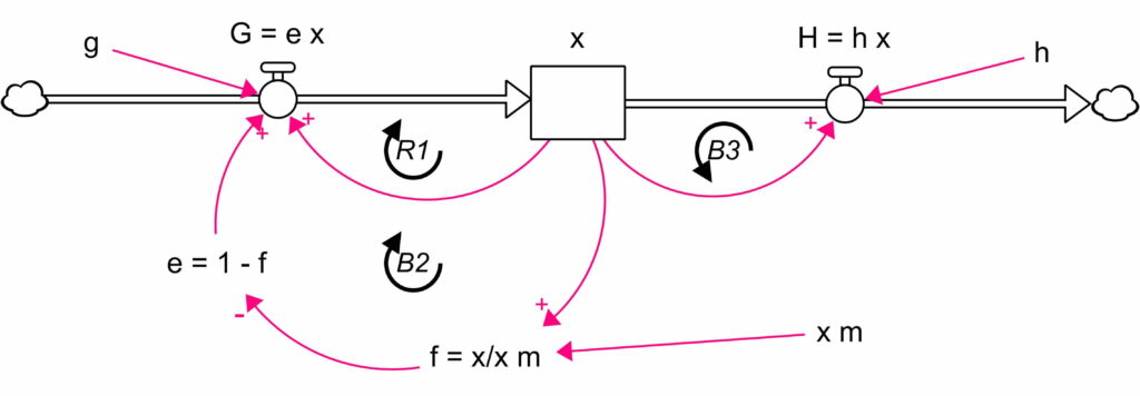
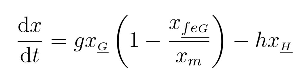
Using the loop impacts (see loop impacts), the differential equation can be converted into a power balance equation that describes how the loops inject and remove energy from the stock. When accumulated, this equation becomes an energy balance equation. Loops are measured by their power (energy per unit time), with changes in the stock represented by the stock’s kinetic energy.
Energy Balance Equation
Using the definition of loop impacts (Loop Impacts equation 6), equation 1 is turned into the power balance equation (Power, equations 3 and 5).
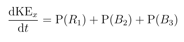
The loop powers, P, are defined by the loop impacts (Power, equation 4). Loop power describes the energy flow into (or out of) a stock. Integrating equation 2 gives the energy balance equation:

where
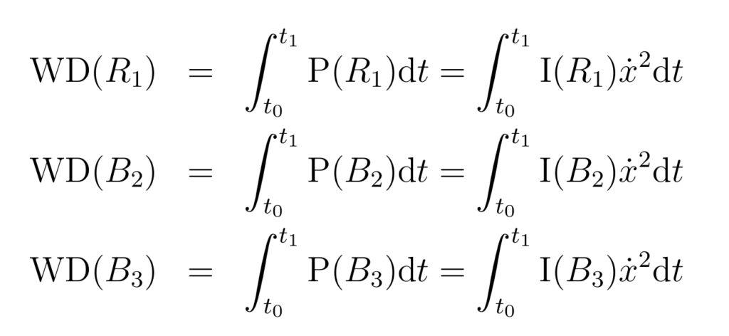
The symbol I represents the impacts of the loops (see loop impacts). WD stands for the “work done” by a loop. That is, the total amount of energy injected, or removed, by the loop between times t0 and t1. Equation 3 is a conservation law. The net amount of energy of the three loops combined is transferred into (or out of) the kinetic energy of the stock, KEx.
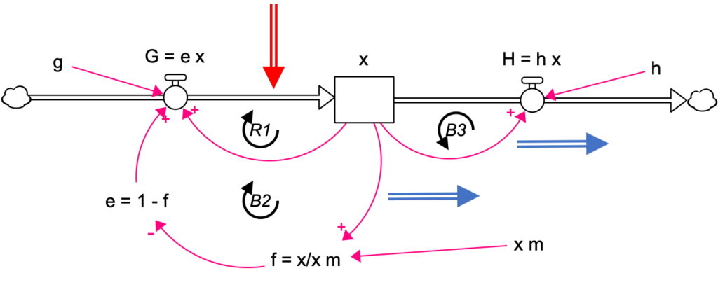
These energy flows can be placed on the stock flow diagram of Figure 1, see Figure 2:
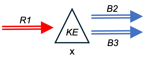
The conservation law, equation 2, can be expressed in diagrammatic form, where the triangle notation represents the kinetic energy of the stock x (Figure 3). This diagram can be viewed as the power balance equation at each point in time (equation 2) or as the energy balance equation integrated over a time interval (equation 3).
Energy Analysis
A graph of the components of the energy balance equation (equation 3) is shown over time, Figure 4. Unlike the power analysis and loop impact analysis, the energy analysis is cumulative. In the early phase, the energy injected by loop R1 is mainly transferred to the stock’s kinetic energy (green curve), with only a small amount removed by the balancing loops. Increasing kinetic energy represents accelerating growth in the stock (Figure 5). In the first 30 years, B2 and B3 have removed about the same amount of energy (red dashed and dotted curves, Figure 4).
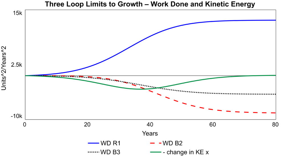
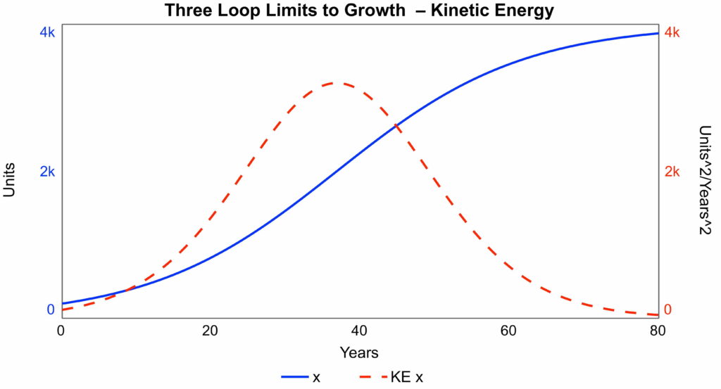
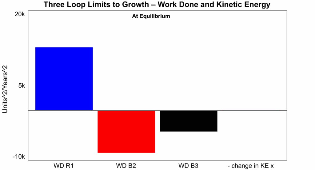
At 38 years, the kinetic energy has peaked (Figures 4 and 5). After this time, B2 has removed more energy than B3, removing twice as much as B3 after 80 years. The energy is removed from both R1 and the stock’s kinetic energy. Hence, the kinetic energy drops to zero, and the stock reaches equilibrium, Figure 5. The final change in kinetic energy is almost zero (Figure 4), as its initial value was relatively small. Over the whole time interval, the diminishing returns loop, B2, has a greater influence on bringing the system to stability than the drain loop, B3.
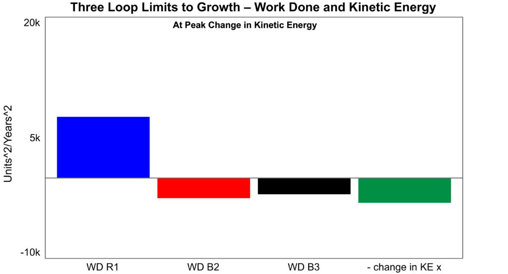
The relative effects of energy injection and removal can be expressed as a bar chart (Figure 6). This chart clearly shows that B2 removes twice as much energy as B3 from the initial value to equilibrium. Figure 7 shows the same comparison up to year 38 when the change in kinetic energy reaches its peak. At this point, the largest amount of energy injected by R1 has been absorbed into the stock’s kinetic energy (green bar). B2 has only removed slightly more than B2. These results depend on the parameter values and the initial value of the stock.
Energy Loss and Equilibrium Value
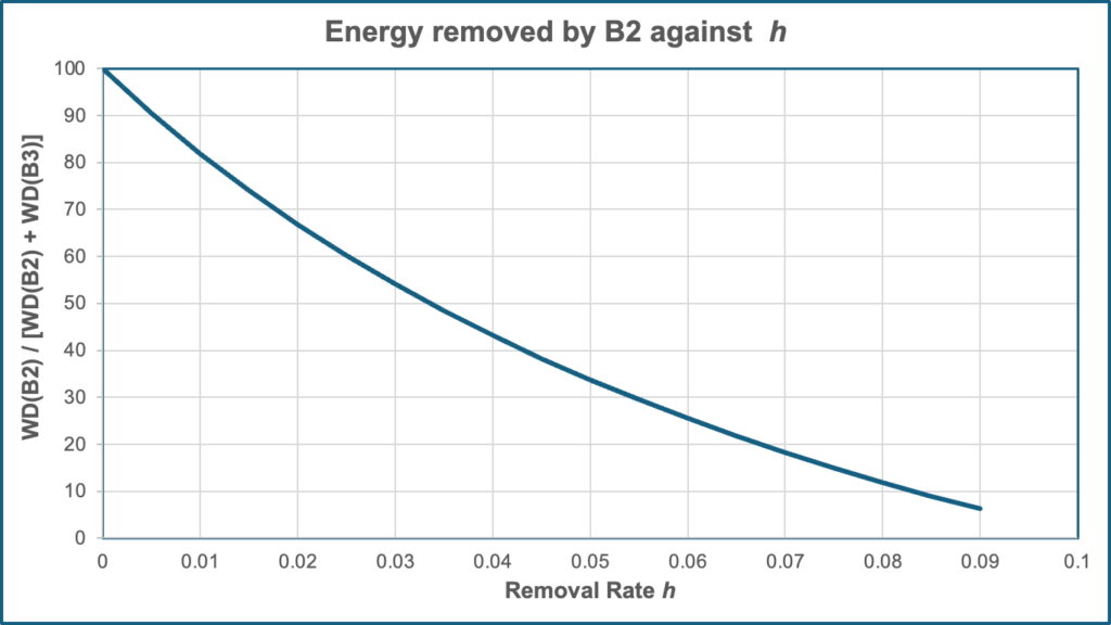
The relative amounts of energy removed by B2 and B3 depend on the parameter values. For example, increasing the removal rate, h, increases the energy removed by loop B3 relative to B2. Figure 8 shows the energy removed by B2 as a percentage of both B2 and B3. When h = 0, B2 removes 100% of the energy to the equilibrium state, indicating that loop B2 is responsible for bringing the system to equilibrium. As h increases, the percentage removed by B2 falls. At h = 0.033, the two loops remove the same amount of energy. For higher values of h, B3 is the main energy remover.
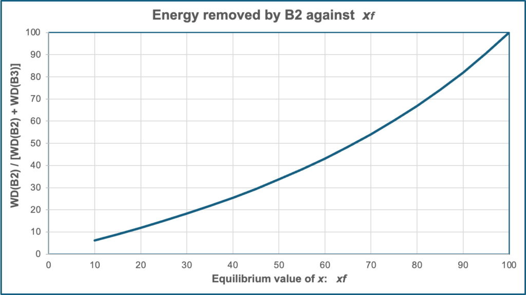
Expressing the percentage energy removed against the equilibrium value of the stock shows that low values of energy removed by B2 are associated with low equilibrium values in the stock (Figure 9). This result indicates that loop B3 determines how far the system falls short of the drain-free equilibrium. The larger the loop B3, the lower the equilibrium value.