The SIR model describes the spread of a disease through a population. The model was originally proposed by Kermack and McKendrick in 1926 using differential equations. However, it can also be presented in system dynamics form using stocks and flows. This modelling style will help clarify the feedback loops.

The population is split into three stocks: Susceptibles (S) – those who are able to catch the disease; Infected (I) – those infected with the disease and capable of passing it on to others; and Removed (R) – those cured of the disease and now immune to further infection, Figure 1. The parameter duration infected is the average length of time a person is infectious. A critical factor in the rate of spread of a disease is the number of people one infected person infects during the period they are infectious. This is referred to as the reproductive ratio and denoted as $R_0$. If $R_0<1$, then the number of infected decreases and the disease dies out. If $R_0>1$, the number of infected increases and an epidemic occurs. The larger $R_0$, the larger the epidemic.

Simulation

The model is simulated starting with a small number of infected people in a population of 67 million, as shown in Figure 2. The growth of the infected starts very slowly – there are only a few thousand infected by the end of week 3. However, it soon accelerates, resulting in 13 million infected by week 9.

The change in the infected stock is controlled by three feedback loops: $R_1$ – a reinforcing loop that controls the uptake of infection; $B_2$ – a balancing loop that controls the depletion of the susceptible population, affecting the infected stock through its inflow; and $B_3$ – a loop that controls the recovery of the infected. Using the Newtonian Interpretative Framework (Hayward & Roach, 2017, 2019), these loops can be thought of as forces that determine the acceleration of the number of infected:

• $R_1$ is a driving force caused by the infected contacting susceptibles;
• $B_2$ is a resistive force due to the depletion of susceptible numbers;
• $B_3$ is another resistive or diffusive force caused by the loss of infected.

Loop Impacts

The influence of these forces can be determined by expressing the stock-flow model as three causally connected differential equations, which preserves the network of connections in Figure 1. Let c stand for the flow catch disease, and r stand for the flow recover. Then $I_c$ is the infected variable along the connector to catch disease, that is, loop $R_1$. By contrast, $I_r$ is the infected variable along the connector to recover, that is $B_3$. Thus, the causal connected differential equations are:

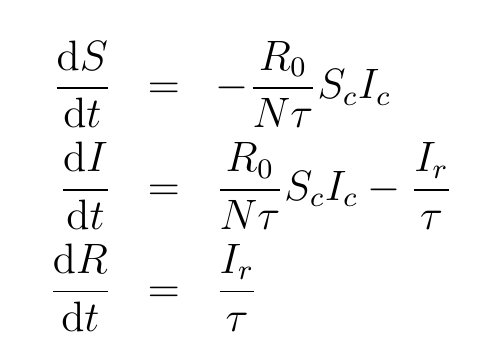
The indices c and r identify the causal path to the stock (variable) with the feedback loops ($R_1$, $B_2$ and $B_3$). The symbol $\tau$ represents the duration infected and N the number of people in the population.

The three forces are measured by the Loop Impact of their respective loops. Loop impact is determined by the ratio of the force’s acceleration to the rate of change of the variable (Hayward & Boswell, 2014). It is a measure of the curvature of the graph of the infected in units per week. The loop impacts are computed by pathway differentiation (Hayward & Roach, 2017, 2019). For the infected:

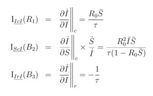
The “bar” indicates the variable is a fraction of the population, e.g.

The notation $\mathrm{I}_{\underline{IcI}}$stands for the impact along the pathway “$I$ catch disease $I$“, that is, loop $R_1$. Note that the loop $B_2$ has an exogenous impact on the infected, $\mathrm{I}_{\underline{ScI}}$. Although “infected” is not in the loop $B_2$, it is nevertheless influenced by the loop.

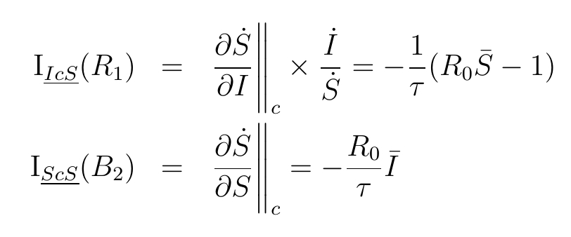
There are two forces on the susceptibles, with impacts:

$B_3$ also has an impact on the Removed, $R$, which is a reaction to the behaviour of the infected.

The loop impacts on infected (equation 2) are plotted in Figure 3.

Force Behaviour

In the first six weeks, $R_1$, the force driving the acceleration of infected, is by far the largest of the three, Figure 3. Although the infected start with a small number and a low rate of change, the driving force has a large impact, Figure 2.

By contrast, the resistive force $B_2$ is initially negligible because the susceptible numbers are well above the epidemic threshold. For the infected to grow:

where $\rho$ is the epidemic threshold, given by the inverse of the reproductive ratio. For $R_0=2.3$, the number infected will increase as long as more than 43% of the population remains susceptible.

The resistive force from $B_3$ has a constant impact as the feedback loop is linear, but it is too small to oppose $R_1$ (Figure 3).

As the number of infections accelerates, the impact of the driving force $R_1$ decreases because the pool of susceptibles shrinks. Correspondingly, the resistive force of the susceptibles $B_2$ increases. Some of the infected’s contacts are with those now in the removed population, who are immune, thereby weakening $R_1$ and strengthening $B_2$. A point is reached at which the combination of the two resistive forces exceeds that of $R_1$, and the increase in the infected slows until its numbers peak. At this point, the infected numbers decrease with $B_2$ accelerating the decline. Both $R_1$ and $B_2$ weaken, leaving the resistive force $B_3$ dominant and slowing the decline of the infected until it reaches zero.

Loop Dominance

The transitions between the infected’s loop impacts (equation 2) are indicated in Figure 4:

When the epidemic ends, some susceptibles remain, having fallen below the threshold (Figure 5). However, with intervention, it is possible to stop the epidemic with fewer people infected, leaving a larger number of susceptibles at the end, at a value up to, but not exceeding, the threshold (in this case, 43%). Interventions correspond to another form of resistive force. Figure 3 indicates that such interventions would be more successful if applied later in the accelerating phase, when the driving force $R_1$ has weakened and the natural resistance of the shrinking susceptible pool, $B_2$, is strong enough to assist the intervention.

An epidemic ends when the number of infected individuals becomes zero, as shown on the susceptible axis in Figure 5. Thus, the entire susceptible axis is in equilibrium. However, only the region below the threshold is stable. The region above the threshold is unstable and therefore cannot be reached without continual interventions, such as quarantine, which would affect the model’s structure, as shown in Figure 1.

References

• Kermack WO and McKendrick AG. 1927. A Contribution to the Mathematical Theory of Epidemics, Proceedings of the Royal Society, A115, 700–21.
• Hayward J and Roach PA. 2017. Newton’s laws as an interpretive framework in system dynamics, System Dynamics Review, 33(3-4), 183–218.
• Hayward J and Roach PA. 2019. The concept of force in population dynamics, Physica A: Statistical Mechanics and its Applications, 531, 121736.
• Hayward J and Boswell GP. 2014. Model behaviour and the concept of loop impact: A practical method. System Dynamics Review, 30(1-2), pp. 29–57.