Kinetic Energy

Energy, a familiar concept in Newtonian mechanics, is a valuable way of describing behaviour in system dynamics models. For example, consider a stock with a constant flow, figure 1:

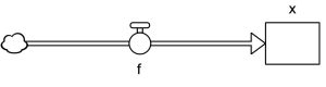
For a positive value of f, stock x increases uniformly over time. The top graph of figure 2 shows its behaviour for an initial value of x =1, with f = 0.2. By time 20, x has become 5 due to accumulation from the flow.

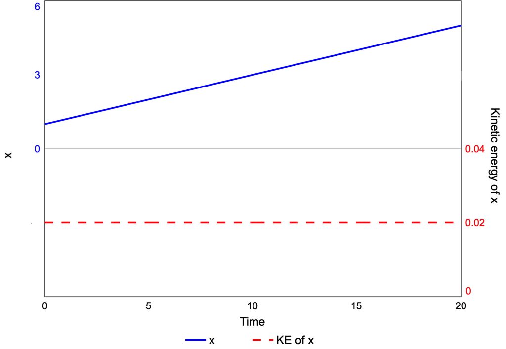
Stock x is changing and can be assigned kinetic energy, similar to a moving particle. In mechanics, kinetic energy is 1/2 mv^2, where m is the mass of a particle and v is its velocity. The net rate of change of a stock is the equivalent of “velocity” if the stock value is thought of as position. But it has no equivalent of mass, for reasons explained later. So I define a stock’s kinetic energy as half its rate of change squared^[1], which for x in figure 1 gives ¹/₂ f².

The bottom graph of figure 2 shows the kinetic energy of x is constant because its rate of change does not vary. Put another way, no forces are acting on stock x to cause its acceleration. That is, there are no stock or exogenous signals influencing x’s flow. Kinetic energy measures activity in a stock.

Energy Sink

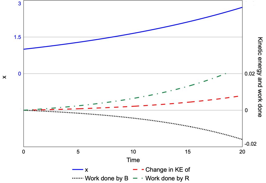
Now place a first-order balancing loop on stock x, figure 3. I interpret loops as a “force” acting on a stock^[2]. This loop is like a frictional force because the larger the stock, the more material is removed. The result is that the uniform growth in x of figure 1 becomes a curve, with x slowing down to reach a limit, figure 4, top graph. Loop B is a decelerating force.

From an energy perspective, loop B is doing work on the stock, reducing its kinetic energy^[3], figure 4 bottom graph. This “work done” is negative, removing energy from the stock. I describe first-order balancing loops as energy sinks^[4]. They play an important role in bringing a system to equilibrium and thus giving control.

The definition of work done is a bit more mathematical and beyond the scope of this post^[5]. However, it is an accumulation measuring how much work is done between the start and end times. Thus, work done describes the loop’s behaviour over the entire time horizon, not just at any point in time.

Energy balances in this system. Notice that the difference between the kinetic energy and B’s work done is constant as they follow the same shaped curve, figure 4. The change in kinetic energy is equal to the work done by B, both negative in this case.

Energy Source

If a first-order balancing loop is an energy sink, then a first-order reinforcing loop is an energy source. Figure 5 has a stock with both types of loops.

If R has a larger gain than B (a>d) then the stock grows and accelerates exponentially, figure 6. Source R puts more energy into the stock than sink B removes. Hence, x increases in kinetic energy, the cause of its acceleration – its upward curvature.

The energy balance equation is: change in kinetic energy of x = work done by R + work done by B.

Units and Dimensions

If stock x has dimensions [X], and time is [T], then the flow has dimensions [X/T]. It follows that kinetic energy and work done have dimensions [X²/T²]. Thus, energy in system dynamics has well-defined units.

Multiple Stocks

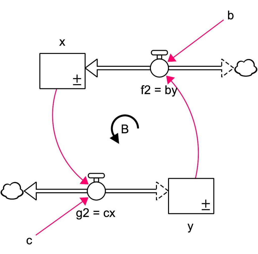
Energy balances in a single stock-flow system if account is taken of the work done by loops and other stocks. In figure 7, stock y does work on stock x, changing the latter’s kinetic energy^[6]. However, energy is not balanced in the whole system. Although y does work on x, x is not doing work on y. Energy balance in stock y must be applied separately to that of x. Indeed, their energies are in different units with insufficient converters to harmonise them.

To balance the energy of the whole system, complete the feedback loop by letting x influence y, e.g. figure 8. This system is fully conserved. The energy injected into y by x balances that injected by x into y. Indeed, second-order balancing loops are the only feedback structure that exchanges energy between stocks in a conserved way^[7].

Had the feedback in figure 8 been an order two reinforcing loop, then that loop would act as a source injecting energy into the whole system. If that source is taken into account, then a single energy balance can still be constructed for the entire system. It contains enough converters to harmonise the energy units of both stocks.

Use of Energy

In our recent paper in the System Dynamics Review, my co-author and I defined energy and applied it to model analysis^[1]. We used the overshoot and collapse model as an example, figure 9. The model contains two stocks. Each has a source and sink, R1 and B1 on Deer, and R2 and B2 on Vegetation. Loop B3 is second-order and exchanges energy between the two stocks. To avoid collapse and achieve a measure of equilibrium, sufficient energy needs to be dissipated overall. In the paper, we show how energy balance can help explain the collapse and suggests modifications to avoid collapse. But that is for another post. In the meantime, read the paper!

References

1. The formal definition of kinetic energy appears in The Concept of Energy in the Analysis of System Dynamics Models. (Hayward J. & Roach P.A., System Dynamics Review, DOI: 10.1002/sdr.1700, 2022).
2. The paper Newton’s Laws as an Interpretive Framework in System Dynamics introduced the concept of force. (Hayward J. & Roach P.A. System Dynamics Review, 33(3-4), 183-218.  DOI: 10.1002/sdr.1586, 2017.)
3. There are two flows in the figure 3 model. The rate of change of x is f-g, giving kinetic energy is 1/2 (f-g)2.
4. See the paper in 1.
5. The paper in 1 gives the formal definition of work done. For first-order loops, it is the integral of the loop impact multiplied by the rate of change squared.
6. We consider the system in figure 7 in papers in 1 and in 2.
7. In the paper in 1, we show an order two balancing loop conserves energy for any non-linearity, regardless of many other structures in the system.

Tags: kinetic energy, source, work done