Diffusion models describe the process by which an entity spreads through a population. Examples include products, technology, ideas, a belief, or an infection. In mathematics, early diffusion models include the Bass model (Bass, 1969) and the Fisher-Pry model (Fisher & Pry, 1971). The model consists of two stocks, often called adopters and potential adopters. For the version here, I will use the SI model that models the spread of a disease through a population where people remain infected permanently. The two stocks are infected and susceptible.
The population is split into two stocks: Susceptibles (S) – those who are able to catch the disease; Infected (I) – those infected with the disease and capable of passing it on to others. The parameter infection rate determines the speed of the diffusion process. The model has one reinforcing loop, R1, and one balancing loop, B1. The loops include the flow catch disease. Thus, both loops affect each stock.

Simulation
The simulation starts with a small number of infected people. Initially, the growth of the infected is slow but continues to accelerate until half the susceptibles become infected, Figure 2, red dashed curve. After that point, the growth slows until. The Diffusion Model is an example of shifting loop dominance. The acceleration phase is dominated by R1 and the decelerating phase by B1. The effects of the loops on the stocks can be quantified by Loop Impact, the ratio that measures the forces between the stocks.

Determining the Forces
The influence of these forces can be determined by expressing the stock-flow model in Figure 1 as two differential equations. The causal connections between the two stocks are expressed by the dependency on S and I, which are unique in this model. The equations are:

The system is one-dimensional due to the conserved flow in Figure 1. Thus, S is determined by algebra from I. The equations give S + I = N, where N is the total population. Differentiating the S equations gives its impacts (Hayward & Boswell, 2014; Hayward & Roach, 2017):
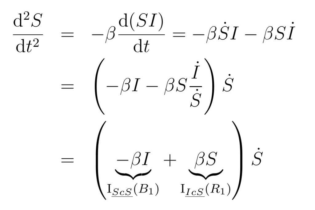
The two impacts indicate the corresponding loop and pathways where c stands for the flow of the disease. Likewise, the impacts on infected I are:

The reinforcing loop has the same impact on each stock. Likewise for loop B1. These results are the expression of the Third Law of Stock Dynamics, which states that in a conserved system, the force on the target stock is equal and opposite to that of the source stock. Because susceptibles are declining and the infected are growing, an extra sign difference appears in the impacts of these forces, making them equal. Thus, the impact analysis is the same for each stock.
Force Behaviour
The two impacts on Infected are plotted in Figure 3. The impact of the force of R1 on Infected falls from 0.5 to zero when there are no more susceptibles, as shown by the blue curve. The impact of B1 is negative. It starts near zero and falls to -0.5. The transition from R1 dominance to B1 dominance occurs when the magnitudes of the impacts are equal at 0.25, producing the dominance pattern in Figure 2.
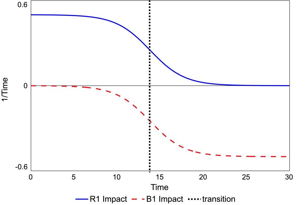
Although the first region has loop R1 dominating behaviour, Figure 3 shows that both loops are always affecting the acceleration of the stocks. Near the transition point, the two loops have similar impacts, and their combination means that acceleration is slight.
This model was discussed in the conference paper Hayward & Roach 2023.
References
- Bass FM 1969. A new product growth model for consumer durables. Management Science 15: 215-227.
- Fisher JC and Pry RH 1971. A simple substitution model of technological change. Technological Forecasting and Social Change 3: 75-88.
- Hayward J and Boswell GP. 2014. Model behaviour and the concept of loop impact: A practical method. System Dynamics Review, 30(1-2), pp. 29–57.
- Hayward J and Roach PA. 2017. Newton’s laws as an interpretive framework in system dynamics, System Dynamics Review, 33(3-4), 183–218.
- Hayward J and Roach PA. 2023. A Comparison of Loop Dominance Methods: Measures and Meaning. Conference version. Presented at the 41st International Conference of the System Dynamics Society, Chicago, July 2023.